Data Flow Analysis in Compilers - Intuition, Equations, and Real Examples
Why Every Compiler Needs Data Flow Analysis: A Simple Overview

Modern compilers don’t optimize code by guesswork.
They optimize by proving facts about programs.
Those facts are computed using Data Flow Analysis (DFA), the backbone of almost every serious compiler optimization.
In this article, we’ll build data flow analysis from first principles:
what it means,
how it works,
and why every optimization pipeline depends on it.
Why Data Flow Analysis Exists?
Consider this code:
x = 5;
y = x + 1;
z = x + 1;
A human immediately sees:
x + 1is computed twiceThe second computation is redundant
A compiler can’t “see” that unless it can prove:
xstill equals5x + 1was already computed earlierNothing in between invalidated it
Data Flow Analysis computes exactly these kinds of facts.
Definition (informal):
Data flow analysis determines what is true about program variables at each point in the program.
Control Flow Graph (CFG): Where DFA Lives
Before analyzing data flow, we need structure.
Compilers convert code into a Control Flow Graph (CFG):
Nodes → basic blocks (straight-line code)
Edges → possible flow of execution
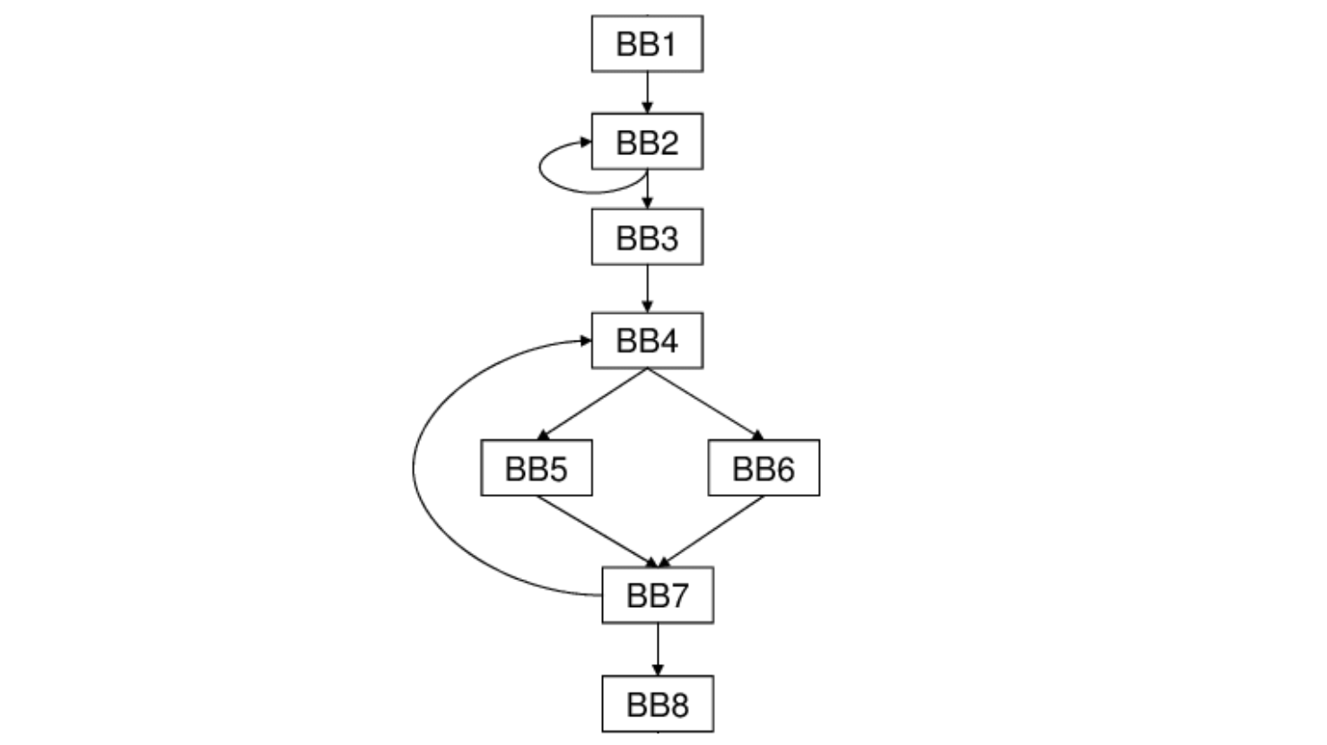
Every data flow analysis runs on the CFG, not directly on source code.
What Is a Data-Flow Fact?
A data-flow fact is information the compiler wants to know at some program point.
Examples:
| Analysis | Data-flow fact |
| Reaching Definitions | Which assignments can reach this point |
| Live Variables | Which variables may be used later |
| Available Expressions | Which expressions are already computed |
| Constant Propagation | Which variables have known constant values |
Different analyses → different facts
Same framework → different meanings
Forward vs Backward Analysis
The direction of analysis depends on where the information flows from.
Forward Analysis
Information flows with execution (entry → exit).
Examples:
Reaching Definitions
Constant Propagation
Available Expressions
Backward Analysis
Information flows against execution (exit → entry).
Examples:
Live Variable Analysis
Very Busy Expressions
Rule of thumb:
If a fact depends on the past → forward
If it depends on the future → backward
With this framework in place, we can look at some of the most common data flow analyses used in real compilers. Each of the following analyses uses the same DFA machinery - only the meaning of the facts changes.
1) Reaching Definitions (RD)
Question it answers:
Which assignments might have produced the current value of a variable?
Data-flow fact:
- A definition (assignment to a variable)
Direction:
- Forward
Meet operator:
- Union (⋃)
Sets:
GEN(b) – definitions created in block
bKILL(b) – other definitions of the same variable
IN(b) – definitions that may reach the start of
bOUT(b) – definitions that may reach after
b
Why it matters:
Enables constant propagation
Enables copy propagation
Explains where values come from
2) Live Variable Analysis (LVA)
Question it answers:
Will this variable be used again in the future?
Data-flow fact:
- A variable
Direction:
- Backward
Meet operator:
- Union (⋃)
Sets:
GEN(b) – variables used before being defined in
bKILL(b) – variables defined in
bIN(b) – variables live at block entry
OUT(b) – variables live at block exit
Why it matters:
Dead code elimination
Register allocation
3) Available Expressions (AE)
Question it answers:
Has this expression already been computed and not invalidated?
Data-flow fact:
- An expression (e.g.,
a + b)
Direction:
- Forward
Meet operator:
- Intersection (⋂)
Sets:
GEN(b) – expressions computed in
bthat surviveKILL(b) – expressions invalidated by assignments in
bIN(b) – expressions available at block entry
OUT(b) – expressions available at block exit
Why it matters:
Common subexpression elimination
Global redundancy elimination
4) Constant Propagation
Question it answers:
Does this variable have a known constant value here?
Data-flow fact:
(variable → constant)mapping
Direction:
- Forward
Meet operator:
Lattice meet (⊓), not simple set union/intersection
Unlike the previous analyses, constant propagation uses a lattice rather than simple set operations, because information can be partially known (for example, unknown vs constant vs conflicting).
Sets (conceptual):
GEN(b) – constant assignments in
bKILL(b) – assignments that overwrite constants
IN(b) – constants known at entry
OUT(b) – constants known at exit
Why it matters:
Eliminates computations
Enables branch simplification
Enables dead code elimination
Seeing these analyses side by side makes the underlying structure of data flow analysis explicit.
A unifying table (this is GOLD)
| Analysis | Fact | Direction | Meet |
| Reaching Definitions | Definition | Forward | ⋃ |
| Live Variables | Variable | Backward | ⋃ |
| Available Expressions | Expression | Forward | ⋂ |
| Constant Propagation | Const mapping | Forward | ⊓ |
Although Reaching Definitions, Live Variables, Available Expressions, and Constant Propagation look different on the surface, they are all instances of the same underlying idea: compute facts, propagate them through control flow, and transform code based on what is proven to be true.
Once this pattern clicks, compiler optimization stops feeling magical and starts feeling systematic.